Microgels

Boyang Zhou

Even though pNipam polymer is charge neutral, charged groups remain on the microgel due to the initiator used for particle synthesis and these cause the formation of an ion-cloud at the particle periphery. One striking effect of pNipam microgel softness is the spontaneous deswelling behavior at high concentrations, where larger particles deswell to the size of smaller ones without direct contact among particles. This behavior results in resolving point defects in the suspension so that crystallization can occur in spite of an initially large polydispersity. Our model for the spontaneous deswelling behavior is that the counter-ion clouds start to percolate when concentration increases. As a result, there are more ‘free’ ions that can contribute to the osmotic pressure. When the osmotic pressure difference becomes larger than the bulk modulus of the particle itself, deswelling occurs. Noting that in pNipam microgel suspensions, the largest microgels are also the softest ones, the largest deswell first when the osmotic pressure increases and in turn the polydispersity is reduced. Thus, our deswelling model describes the change of polydispersity due to deswelling and this relates particle softness with phase behavior. Therefore, the characterization of the counter-ion cloud is key to understand the phase behavior at high concentrations.

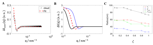
Figure 1: (A) The cloud signal extracted with sodium and ammonium-ion samples and is fitted by the model in (B). (B) spherical shell model with shell radius R_ic and width σ_ic plotted in the Fourier space with increasing R_ic and fixed σ_ic (black: large R_ic. Blue: small R_ic). (C) Particle radii plotted over increasing ζ. (R_sans = R_c + 2*σ_s)

We use small-angle neutron scattering (SANS) to reveal the signal due to the counterion cloud by taking the difference between two samples that contain the same microgels at the essentially same number densities but in the presence of different counterions, sodium (Na⁺) or ammonium (NH₄⁺). Suspensions containing either ion can be obtained using dialysis. By directly subtracting scattering intensity of Na⁺ sample from that of NH₄⁺ sample with number density corrections, we successfully revealed the cloud signal that can be modeled with a spherical shell in the Fourier space, Fig.1. Our results corroborate our expectations that the counterion cloud is located at the particle surface with a width around 40nm. To further demonstrate our theory, we prepared microgel suspension with increasing volume fraction ζ and used SANS to track the particle radii. We observed a plateau of R_sans at low ζ and observed the spontaneous deswelling of particle before the concentration reaches the random close packing density ζ=0.64. By calculating the true volume fraction ϕ^True =ζ((R_sans (ζ))/R_swollen )³ and effective volume fractions ϕ^eff=ζ((R_sans (ζ)+ΔR)/R_swollen )³ and ζ^eff=ζ((R_swollen+ΔR)/R_swollen )³, where ΔR is the counterion cloud width, we can have an estimation of cloud width when particles just start to spontaneously deswell, Fig.2.

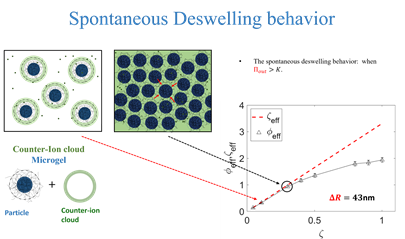
At ζ_eff=ϕ_eff=1, particles with radius of R_sans+ΔR occupy all the space in the suspension with percolation of the cloud, which subsequently creates a higher osmotic pressure outside of the particle Π_out. When this pressure is larger than the bulk modulus of the particle K, the particles get isotropically compressed (red arrow). With this method, we also get the cloud width in the range of 40nm, a reproduceable result from our direct measurements with SANS. Since contributions to osmotic equilibrium due to polymer-solvent mixing and network elasticity are largely independent of suspension concentration, ionic effects turn out to be key to understand the suspension behavior; while at low particle densities free ions can wander inside and outside the microgels, at high particle densities, the overlap of counterion clouds can cause the outside osmotic pressure to increase and to induce deswelling. As a result, any model or simulation aiming to capture the phase behavior and mechanics of nearly all microgel suspensions, which are based on either network-charged or peripherically-charged microgels, should explicitly consider the effect of ions.

Microgels: dense suspensions

Adrian Arenas Gullo

The dynamics of a microgel suspension is highly influenced by particle concentration. In colloidal systems, the volume fraction, 𝜙, acts as the inverse of temperature would in atomic systems. Instead of 𝜙, we use the generalized volume fraction, ζ, since it gets hardly possible to calculate 𝜙 when the microgel particles can shrink and deform.

In order to study the dynamics of pNIPAM microgels, we perform 3D Dynamic Light Scattering experiments, where we measure the intensity of laser beams that go through the sample. The difference in permitivity between water and gel particles cause the laser photons to scatter, giving rise to fluctuations in the intensity detection. Then, we can calculate the intensity correlation as a function of lag-time, which is related to the electric field correlation via the Siegert relation [1]. Its normalized version, including a correction K, reads as: 𝑔_𝐼(𝑞,𝜏)−1=𝐾|𝑔_𝐸 (𝑞,𝜏)|².

The parameter K(≤1) gives the signal to noise ratio, including misalignments in the setup, as well as signal lost because of multiple scattering events. The intensity correlation decays with lag time, as measurements tend to lose there relation as the time between events grows higher. In a monodisperse system of diffusive particles undergoing Brownian motion, the field correlation decays exponentially. Its expression, along with the Stokes-Einstein equation can then be used to infer the hydrodynamic radius of the particles, 𝑅_h: |𝑔_𝐸(𝑞,𝜏)|=exp(−𝐷𝑞^² 𝜏) ; 𝑅_ℎ=(𝑘_𝐵 𝑇)/(6𝜋𝜂_𝑠 𝐷).

Assuming we know the solvent viscosity, we can perform experiments at different angles to do a linear regression. At each angle, we can define the relaxation time (or frequency): 𝜏0=(𝐷𝑞² )⁽⁻¹⁾=(Γ₀ )⁽⁻¹⁾. If the system if concentrated, the correlation dependence on lag time isn’t that simple. Instead, it shows a first decay, associated to particles jiggling, and a second one, at longer times, associated the particles escaping their cage. We note the structural time relaxation associated to this decay by τ_α. The long time decay is well described by a stretched exponential [2]: 𝑔_𝐼−1 ∝ exp(−2(𝜏/𝜏_𝛼 )^𝛽 ).

Our pNIPAM microgel is responsive to changes in temperature and pH, affecting its affinity with water. A low temperature and high pH will result in a swollen gel, while the opposite conditions will make it shrink. pNIPAM is known to undergo a LCST phase transition around 32°C. These changes in solute-solvent interaction are described by Flory-Rehner theory. Since we want to use the “same system” at all moment, we only change the volume fraction of our hydrogel.

However, this change has a huge effect in the dynamics of the system. In the diffusive limit, we have τ₀∼1 s. However, for the highest volume fractions, we get a final decay characterized by τ_α, which is 3 or 4 orders of magnitude higher than τ₀. This fact is slightly inconvenient for the data acquisition. The equipment we use calculates g_I using a correlator, which allows us to sample at τ∼10^(-8)s. However, its maximum sample time is limitted too. Since the detector records the count rate history, with a sample time t_S, we can reconstruct g_I for τ=n t_S. We use both versions of the correlation function, showing how they overlap in the middle range.

Another important detail to mention is that, when studying the decorrelation of this system, it’s generally more visual to represent times logarithmically. In fact, the correlator space its results pseudo-logarithmically. When we try to fit the data to a particular functional form, this spacing ensures that the fit isn’t biased towards the longer times (for which there would be more data if the spacing was linear), where the noise is bigger. 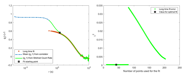Because of that, we restrict the values for this second correlation function to a logarithmically spaced set. Lastly, we want to fit the long time correlation function. To do that in a methodic way, we construct fits going from one point to the last and calculate χ^2 to estimate the error of the fit. We repeat this changing the starting point, and select the fit that minimizes the error.

As we can see, the fit starts after the first “decorrelation step” has taken place. The shortest time value is around 2.5 s, and we obtain the relaxation time τ_α=(4.4±0.4)·10³ s.

[1] Dhont, J. K. G. (1996). An Introduction to Dynamics of Colloids, Elsevier
[2] Philippe, A. M., Truzzolillo, D., Galvan-Myoshi, J., Dieudonné-George, P., Trappe, V., Berthier, L., & Cipelletti, L. (2018). Glass transition of soft colloids. Physical Review E, 97(4), 1–5.